Technical Guide
This document describes the technical details of the competition framework for the F1TENTH Sim Racing League. It goes over the details pertaining to the simulator and devkit, as well as some important aspects of the submission system, process, and evaluation.
Warning
It expected that teams have sufficient background knowledge pertaining to autonomous racing (concepts, methods, and algorithms), programming languages (Python, C++, etc.) and frameworks (ROS 2), containerization (Docker) and version control (Git), etc. In order to be fair to all teams and keep the competition on schedule, extensive technical support/help cannot be provided by the organizers. However, legitimate requests may be entertained at the discretion of the organizers.
Note
Although AutoDRIVE Ecosystem supports various vehicles across different scales, configurations, and operational design domains (ODDs), the only vehicle allowed for this competition is the F1TENTH. Similarly, although AutoDRIVE Ecosystem supports multiple application programming interfaces (APIs), the only API allowed for this competition is ROS 2.
Please see the accompanying video for a step-by-step tutorial of setting up and using the competition framework.
1. AutoDRIVE Simulator
AutoDRIVE Simulator (part of the larger AutoDRIVE Ecosystem) is an autonomy oriented tool designed to model and simulate vehicle and environment digital twins. It equally prioritizes backend physics and frontend graphics to achieve high-fidelity simulation in real-time. From a computing perspective, the simulation framework is completely modular owing to its object-oriented programming (OOP) constructs. Additionally, the simulator can take advantage of CPU multi-threading as well as GPU instancing (if available) to efficiently parallelize various simulation objects and processes, with cross-platform support.
For the F1TENTH Sim Racing League, each team will be provided with a standardized simulation setup (in the form of a digital twin of the F1TENTH vehicle, and a digital twin of the Porto racetrack) within the high-fidelity AutoDRIVE Simulator. This would democratize autonomous racing and make this competition accessible to everyone across the globe.
1.1. System Requirements
Minimum Requirements:
- Platform: Ubuntu 20.04+, Windows 10+, macOS 10.14+ (simulator has cross-platform compatibility)
- Processor: Quad-core CPU (e.g., Intel Core i5 or AMD Ryzen 5)
- Memory: 8 GB RAM
- Graphics: Integrated graphics (e.g., Intel HD Graphics) or a low-end discrete GPU (e.g., NVIDIA GeForce GTX 1050) with at least 2 GB of VRAM
- Storage: 10 GB of free disk space (for storing Docker images, simulator application and data)
- Display: 1280x720 px resolution with 60 Hz refresh rate
- Network: Stable internet connection (1 Mbps) for pulling/pushing Docker images, and downloading updates on demand
Recommended Requirements:
- Platform: Ubuntu 20.04/22.04, Windows 10/11 (simulator has been extensively tested on these platforms)
- Processor: Octa-core CPU (e.g., Intel Core i7 or AMD Ryzen 7)
- Memory: 16 GB RAM
- Graphics: Mid-range discrete GPU (e.g., NVIDIA GeForce GTX 1660 or RTX 2060) with 4+ GB of VRAM
- Storage: 20 GB of free disk space (to accommodate multiple Docker images, additional data, and logs)
- Display: 1920x1080 px resolution with 144 Hz refresh rate
- Network: Fast internet connection (10 Mbps) for pulling/pushing Docker images, and downloading updates on the fly
Info
Note that the organizers will execute the competition framework on a workstation incorporating Intel Core i9 14th Gen 14900K CPU, NVIDIA GeForce RTX 4090 GPU, and 64 GB RAM (or a similar configuration). This machine will be simultaneously running the simulator container, devkit container, screen recorder and data logger. Kindly develop your algorithms while considering these computational requirements.
1.2. User Interface
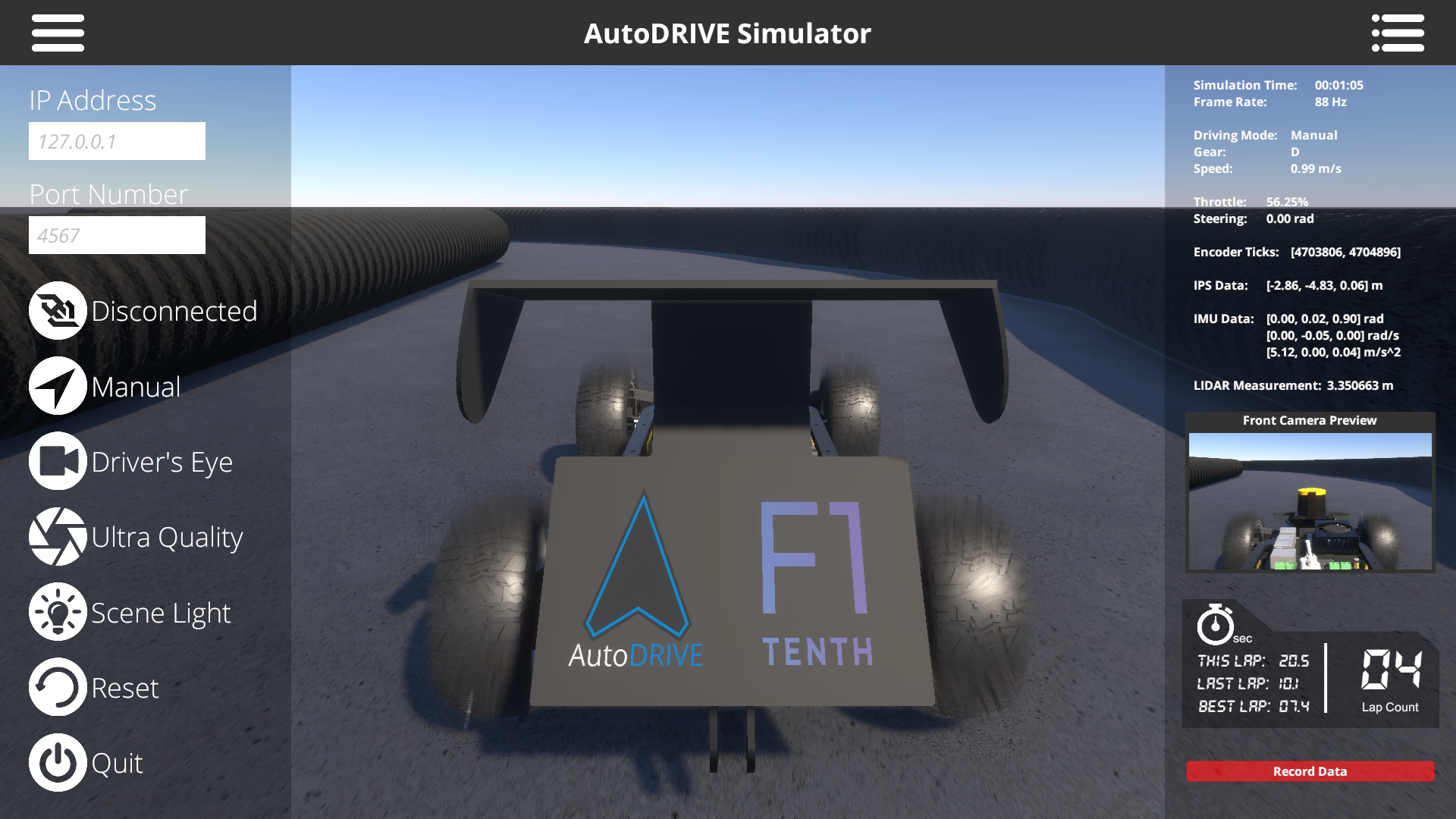
AutoDRIVE Simulator's graphical user interface (GUI) consists of a toolbar encompassing two panels for observing and interacting with key aspects of the simulator in real-time, namely Menu and Heads-Up Display (HUD). Both the panels can be enabled or disabled using the burger icons provided on the toolbar; the figure above illustrates both the GUI panels being enabled. The menu panel on the left-hand side helps configure and control some important aspects of the simulation with just a few clicks. The HUD panel on the right-hand side helps visualize prominent simulation parameters along with vehicle status and sensory data, while hosting a time-synchronized data recording functionality that can be used to export simulation data for a specific run.
1.2.1. Menu Panel
- IP Address Field: Input field to specify IP address for the machine running the devkit (default is 127.0.0.1, i.e., standard address for IPv4 loopback traffic).
- Port Number Field: Input field to specify port number for the machine running the devkit (default is 4567, observed to be usually unoccupied).
- Connection Button: Button to establish connection with the devkit, which acts as the server with the simulator being the client (the button is disabled once the connection is established). The status of bridge connection (i.e., Connected or Disconnected) is displayed besides this button.
- Driving Mode Button: Button to toggle the driving mode of the vehicle between Manual and Autonomous (default is Manual). The selected driving mode is displayed besides this button.
- Camera View Button: Button to toggle the scene camera view between Driver’s Eye, Bird’s Eye and God’s Eye (default is Driver’s Eye). The selected view is displayed besides this button.
- Graphics Quality Button: Button to toggle the graphics quality view between Low, High, and Ultra (default is Low). The selected quality is displayed besides this button.
- Scene Light Button: Button to enable/disable the environmental lighting (default is enabled).
- Reset Button: Button to reset the simulator to initial conditions.
- Quit Button: Button to quit the simulator application.
1.2.2. HUD Panel
- Simulation Time: The time (HH:MM:SS) since start of the simulation. Reset button resets the simulation time.
- Frame Rate: Running average of the FPS value (Hz).
- Driving Mode: Driving mode of the ego-vehicle (Manual or Autonomous).
- Gear: Driving gear of the vehicle, either Drive (D) or Reverse (R).
- Speed: Magnitude of forward velocity of the vehicle (m/s).
- Throttle: Instantaneous throttle input of the vehicle (%).
- Steering: Instantaneous steering angle of the vehicle (rad).
- Encoder Ticks: Ticks (counts) of the rear-left and rear-right incremental encoders of the vehicle represented using a 1D array of 2 elements [left_ticks, right_ticks].
- IPS Data: Position (m) of the vehicle within the environment represented using a 1D vector [x, y, z].
- IMU Data: Orientation [x, y, z] rad, angular velocity [x, y, z] rad/s, and linear acceleration [x, y, z] m/s2 of the ego-vehicle w.r.t. body frame of reference.
- LIDAR Measurement: Instantaneous ranging measurement (m) of the 270° FOV 2D LIDAR on the vehicle.
- Camera Preview: Instantaneous raw image from the front camera of the vehicle.
- Race Telemetry: Current elapsed lap time (s), last lap time (s), overall best lap time (s) as well as total lap count data.
- Data Recorder: Save time-synchronized simulation data for a specific simulation run.
1.2.3. Data Recorder
AutoDRIVE Simulator hosts a time-synchronized data recording functionality that can be used to export simulation data at 30 Hz. The data is saved in CSV format and the raw camera frames are exported as timestamped JPG files. The CSV file hosts the following data entries per timestamp:
| DATA | timestamp | throttle | steering | leftTicks | rightTicks | posX | posY | posZ | roll | pitch | yaw | speed | angX | angY | angZ | accX | accY | accZ | camera | lidar |
|---|---|---|---|---|---|---|---|---|---|---|---|---|---|---|---|---|---|---|---|---|
| UNIT | yyyy_MM_dd_HH_mm_ss_fff | norm% | rad | count | count | m | m | m | rad | rad | rad | m/s | rad/s | rad/s | rad/s | m/s^2 | m/s^2 | m/s^2 | img_path | array(float) |
The data recorder can be triggered by clicking on the red Record Data button in the HUD panel, or using the R hotkey. The first time, the data recorder will prompt the user to specify the directory path to store the data. The second trigger will start recording the data, which can be verified by checking the status of the red button change from Record Data to Recording Data. Finally, the third trigger will stop data recording, which can be verified by checking the status of the red button change from Recording Data to Saving Data with the save percentage being displayed.
Info
When specifying the directory path to store the data, just select the directory where you want the data to be saved with a single click, do not enter that directory by double-clicking onto it.
Warning
Although the data is meant to be recorded at 30 Hz, the actual rate depends on the compute power and the OS schedular, and may therefore fluctuate a bit. However, the data will still be time-synchronized.
Note
If you try to record data two (or more) times in a row, without resetting or restarting the simulator, the new data will be appended to the same CSV file and the new camera frames will be added to the same Camera Frames directory. The old data will not be overwritten for user convenience and one can differentiate between the old and new datasets using the timestamp variable. However, if this is not intended, please consider resetting or restarting the simulator and specifying a different directory to store the new data.
1.3. Vehicle
Simulated vehicles can be developed using AutoDRIVE's modular scripts, or imported from third-party tools and open standards. Specifically, the F1TENTH vehicle was reverse-engineered and visually recreated using a third-party 3D modeling software, and was imported and post-processed within AutoDRIVE Simulator to make it physically and graphically "sim-ready".
These vehicles are simulated as a combination of rigid body and sprung mass representations with adequate attention to rigid body dynamics, suspension dynamics, actuator dynamics, and tire dynamics. Additionally, the simulator detects mesh-mesh interference and computes contact forces, frictional forces, momentum transfer, as well as linear and angular drag acting on the vehicle. Finally, being an autonomy-oriented digital twin, the simulator offers physically-based sensor simulation for proprioceptive as well as exteroceptive sensors on-board the virtual vehicle.
1.3.1. Transforms
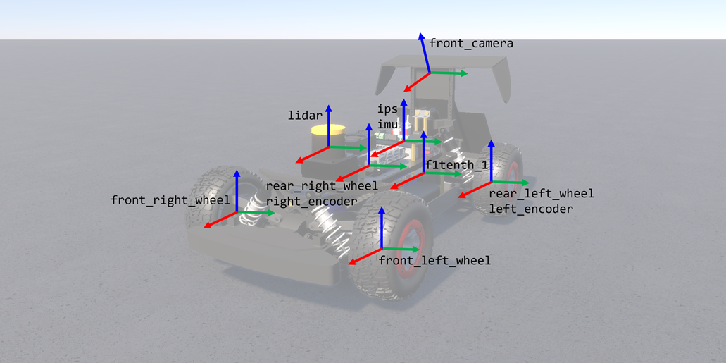
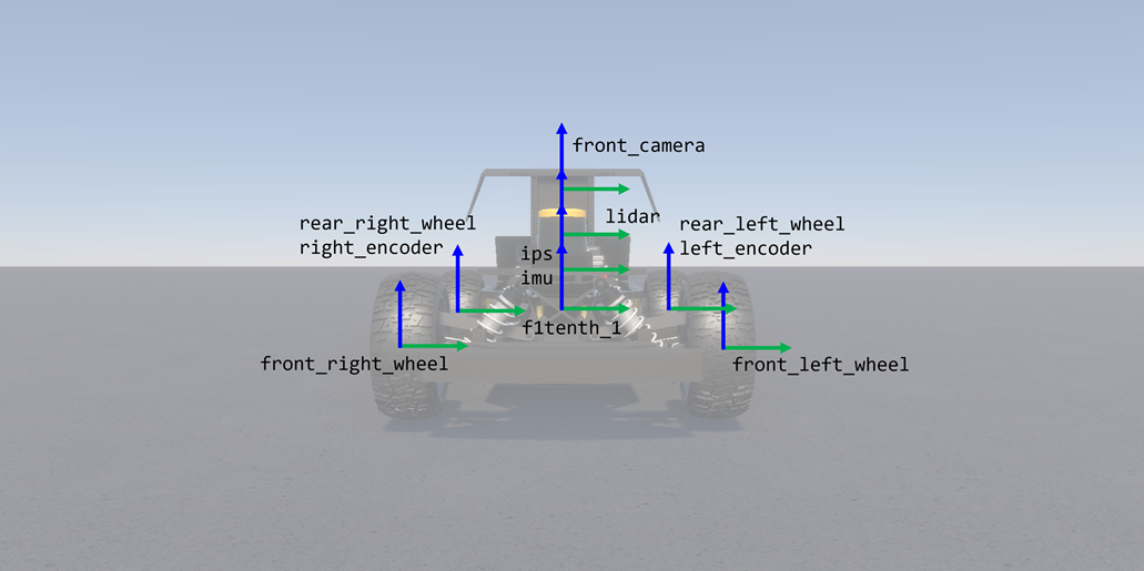
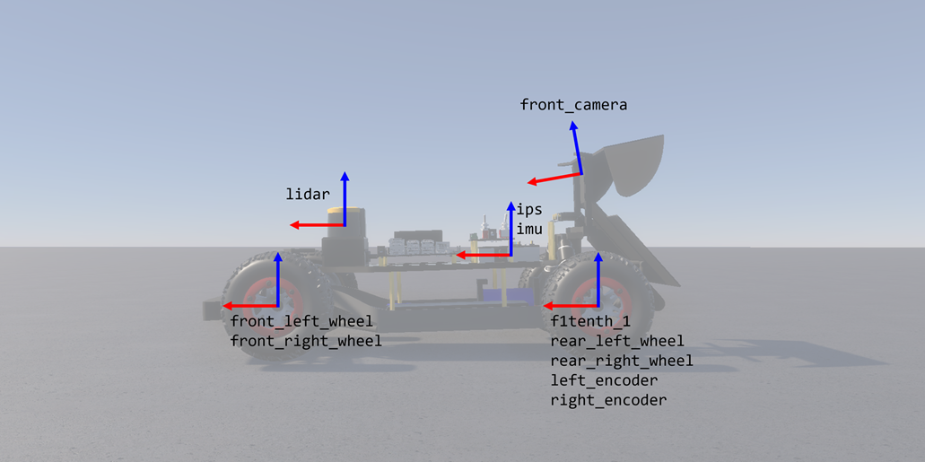
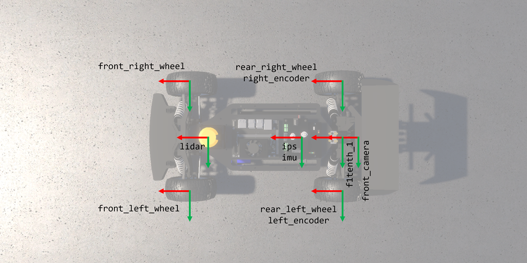
Note
All right-handed coordinate frames depicted above are defined such that red represents x-axis, green represents y-axis, and blue represents z-axis.
| FRAME | x | y | z | R | P | Y |
|---|---|---|---|---|---|---|
left_encoder |
0.0 | 0.118 | 0.0 | 0.0 | 0.0 | |
right_encoder |
0.0 | -0.118 | 0.0 | 0.0 | 0.0 | |
ips |
0.08 | 0.0 | 0.055 | 0.0 | 0.0 | 0.0 |
imu |
0.08 | 0.0 | 0.055 | 0.0 | 0.0 | 0.0 |
lidar |
0.2733 | 0.0 | 0.096 | 0.0 | 0.0 | 0.0 |
front_camera |
-0.015 | 0.0 | 0.15 | 0.0 | 10.0 | 0.0 |
front_left_wheel |
0.33 | 0.118 | 0.0 | 0.0 | 0.0 | |
front_right_wheel |
0.33 | -0.118 | 0.0 | 0.0 | 0.0 | |
rear_left_wheel |
0.0 | 0.118 | 0.0 | 0.0 | 0.0 | |
rear_right_wheel |
0.0 | -0.118 | 0.0 | 0.0 | 0.0 |
Note
All frame transforms mentioned above are defined w.r.t. the vehicle (local) frame of reference f1tenth_1 located at the center of rear axle with x-axis pointing forward, y-axis pointing left, and z-axis pointing upwards. Columns x, y, and z denote translations in meters (m), while R, P, and Y denote rotations in degrees (deg). denotes variable quantities.
1.3.2. Vehicle Dynamics
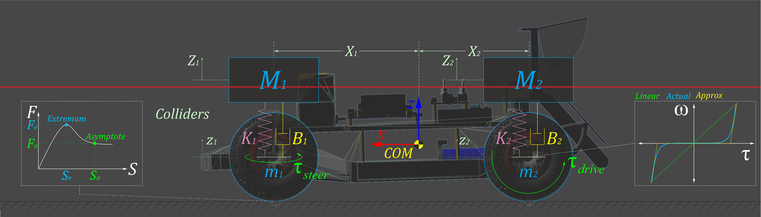
The vehicle model is a combination of a rigid body and a collection of sprung masses \(^iM\), where the total mass of the rigid body is defined as \(M=\sum{^iM}\). The rigid body's center of mass, \(X_{COM} = \frac{\sum{{^iM}*{^iX}}}{\sum{^iM}}\), connects these representations, with \(^iX\) representing the coordinates of the sprung masses.
The suspension force acting on each sprung mass is computed as \({^iM} * {^i{\ddot{Z}}} + {^iB} * ({^i{\dot{Z}}}-{^i{\dot{z}}}) + {^iK} * ({^i{Z}}-{^i{z}})\), where \(^iZ\) and \(^iz\) are the displacements of sprung and unsprung masses, and \(^iB\) and \(^iK\) are the damping and spring coefficients of the \(i\)-th suspension, respectively. The unsprung mass \(m\) is also subject to gravitational and suspension forces: \({^im} * {^i{\ddot{z}}} + {^iB} * ({^i{\dot{z}}}-{^i{\dot{Z}}}) + {^iK} * ({^i{z}}-{^i{Z}})\).
Tire forces are computed based on the friction curve for each tire, represented as \(\left\{\begin{matrix} {^iF_{t_x}} = F(^iS_x) \\{^iF_{t_y}} = F(^iS_y) \\ \end{matrix}\right.\), where \(^iS_x\) and \(^iS_y\) are the longitudinal and lateral slips of the \(i\)-th tire, respectively. The friction curve is approximated using a two-piece cubic spline, defined as \(F(S) = \left\{\begin{matrix} f_0(S); \;\; S_0 \leq S < S_e \\ f_1(S); \;\; S_e \leq S < S_a \\ \end{matrix}\right.\), where \(f_k(S) = a_k*S^3+b_k*S^2+c_k*S+d_k\) is a cubic polynomial function. The first segment of the spline ranges from zero \((S_0,F_0)\) to an extremum point \((S_e,F_e)\), while the second segment ranges from the extremum point \((S_e, F_e)\) to an asymptote point \((S_a, F_a)\).
The tire slip is influenced by factors including tire stiffness \(^iC_\alpha\), steering angle \(\delta\), wheel speeds \(^i\omega\), suspension forces \(^iF_s\), and rigid-body momentum \(^iP\). These factors impact the longitudinal and lateral components of the vehicle's linear velocity. The longitudinal slip \(^iS_x\) of \(i\)-th tire is calculated by comparing the longitudinal components of the surface velocity of the \(i\)-th wheel \(v_x\) with the angular velocity \(^i\omega\) of the \(i\)-th wheel: \({^iS_x} = \frac{{^ir}*{^i\omega}-v_x}{v_x}\). The lateral slip \(^iS_y\) depends on the tire's slip angle \(\alpha\) and is determined by comparing the longitudinal \(v_x\) and lateral \(v_y\) components of the vehicle's linear velocity: \({^iS_y} = \tan(\alpha) = \frac{v_y}{\left| v_x \right|}\).
| VEHICLE PARAMETERS | |
|---|---|
| Car Length | 0.5000 m |
| Car Width | 0.2700 m |
| Wheelbase | 0.3240 m |
| Track Width | 0.2360 m |
| Front Overhang | 0.0900 m |
| Rear Overhang | 0.0800 m |
| Wheel Radius | 0.0590 m |
| Wheel Width | 0.0450 m |
| Total Mass | 3.906 kg |
| Sprung Mass | 3.470 kg |
| Unsprung Mass | 0.436 kg |
| Center of Mass | X: 0.15532 m Y: 0.00000 m Z: 0.01434 m |
| Suspension Spring | 500 N/m |
| Suspension Damper | 100 Ns/m |
| Longitudinal Tire Limits (Slip, Force) | Extremum: (0.15, 0.72) Asymptote: (0.25, 0.464) |
| Lateral Tire Limits (Slip, Force) | Extremum: (0.01, 1.00) Asymptote: (0.10, 0.500) |
1.3.3. Actuator Dynamics
The driving actuators apply torque to the wheels: \({^i\tau_{drive}} = {^iI_w}*{^i\dot{\omega}_w}\), where \({^iI_w} = \frac{1}{2}*{^im_w}*{^i{r_w}^2}\) represents the moment of inertia, \(^i\dot{\omega}_w\) is the angular acceleration, \(^im_w\) is the mass, and \(^ir_w\) is the radius of the \(i\)-th wheel. Additionally, the driving actuators simulate idle torque by applying an equivalent braking torque, i.e., \({^i\tau_{idle}} = {^i\tau_{brake}}\).
| DRIVING ACTUATOR | |
|---|---|
| Drive Type | All wheel drive |
| Throttle Limits | [-1,1] |
| Motor Torque | 428 Nm |
| Vehicle Top Speed | 22.88 m/s |
The front wheels are steered at the commanded steering angle \(\delta\) using a steering actuator. The individual turning angles, \(\delta_l\) and \(\delta_r\), for the left and right wheels, respectively, are computed based on the Ackermann steering geometry defined by the wheelbase \(l\) and track width \(w\), as follows: \(\left\{\begin{matrix} \delta_l = \textup{tan}^{-1}\left(\frac{2*l*\textup{tan}(\delta)}{2*l+w*\textup{tan}(\delta)}\right) \\ \delta_r = \textup{tan}^{-1}\left(\frac{2*l*\textup{tan}(\delta)}{2*l-w*\textup{tan}(\delta)}\right) \end{matrix}\right.\)
| STEERING ACTUATOR | |
|---|---|
| Steer Type | Ackermann steering |
| Steering Limits | [-1,1] |
| Steering Angle Limits | [-0.5236,0.5236] rad |
| Steering Rate | 3.2 rad/s |
1.3.4. Sensor Physics
Throttle (\(\tau\)) and steering (\(\delta\)) sensors are simulated using an instantaneous feedback loop. Incremental encoders are simulated by measuring the rotation of the rear wheels: \(^iN_{ticks} = {^iPPR} * {^iCR} * {^iN_{rev}}\), where \(^iN_{ticks}\) and \(^iPPR\) respectively represent the measured ticks and base resolution (pulses per revolution) of the \(i\)-th encoder, while \(^iCR\) and \(^iN_{rev}\) respectively represent the conversion ratio and output shaft revolutions of the \(i\)-th motor.
| THROTTLE SENSOR | |
|---|---|
| Type | Virtual Sensor |
| Class | Actuator Feedback |
| Supported Outputs | [-1, 1] |
| STEERING SENSOR | |
|---|---|
| Type | Virtual Sensor |
| Class | Actuator Feedback |
| Supported Outputs | [-1, 1] |
| ENCODERS | |
|---|---|
| Type | Simulated Sensor |
| Class | Proprioceptive |
| Pulses Per Revolution | 16 |
| Conversion Ratio | 120 |
| Supported Outputs | Ticks Angles |
The indoor positioning system (IPS) and inertial measurement unit (IMU) are simulated based on temporally-coherent rigid-body transform updates of the vehicle \(\{v\}\) w.r.t. the world \(\{w\}\): \({^w\mathbf{T}_v} = \left[\begin{array}{c | c} \mathbf{R}_{3 \times 3} & \mathbf{t}_{3 \times 1} \\ \hline \mathbf{0}_{1 \times 3} & 1 \end{array}\right] \in SE(3)\). IPS provides 3-DOF positional coordinates \(\{x,y,z\}\) of the vehicle, while IMU supplies linear accelerations \(\{a_x,a_y,a_z\}\), angular velocities \(\{\omega_x,\omega_y,\omega_z\}\), and 3-DOF orientation of the vehicle as Euler angles \(\{\phi_x,\theta_y,\psi_z\}\) or quaternion \(\{q_0,q_1,q_2,q_3\}\).
| IPS | |
|---|---|
| Type | Simulated Sensor |
| Class | Proprioceptive |
| Supported Outputs | Position Vector [x, y, z] m |
| IMU | |
|---|---|
| Type | Simulated Sensor |
| Class | Proprioceptive |
| Supported Outputs | Orientation Quaternion [x, y, z, w] Orientation Euler Angles [x, y, z] rad Angular Velocity Vector [x, y, z] rad/s Linear Acceleration Vector [x, y, z] m/s2 |
LIDAR simulation employs iterative ray-casting \(\texttt{raycast}\){\(^w\mathbf{T}_l\), \(\vec{\mathbf{R}}\), \(r_{max}\)} for each angle \(\theta \in \left [ \theta_{min}:\theta_{res}:\theta_{max} \right ]\) at a specified update rate. Here, \({^w\mathbf{T}_l} = {^w\mathbf{T}_v} \times {^v\mathbf{T}_l} \in SE(3)\) represents the relative transformation of the LIDAR {\(l\)} w.r.t the vehicle {\(v\)} and the world {\(w\)}, \(\vec{\mathbf{R}} = \left [\cos(\theta) \;\; \sin(\theta) \;\; 0 \right ]^T\) defines the direction vector of each ray-cast, \(r_{min}\), \(r_{max}\), \(\theta_{min}\) and \(\theta_{max}\) denote the minimum and maximum linear and angular ranges, and \(\theta_{res}\) represents the angular resolution of the LIDAR. The laser scan ranges are determined by checking ray-cast hits and then applying a threshold to the minimum linear range of the LIDAR, calculated as \(\texttt{ranges[i]}=\begin{cases} d_\text{hit} & \text{ if } \texttt{ray[i].hit} \text{ and } d_\text{hit} \geq r_{\text{min}} \\ \infty & \text{ otherwise} \end{cases}\), where \(\texttt{ray.hit}\) is a Boolean flag indicating whether a ray-cast hits any colliders in the scene, and \(d_\text{hit}=\sqrt{(x_{\text{hit}}-x_{\text{ray}})^2 + (y_{\text{hit}}-y_{\text{ray}})^2 + (z_{\text{hit}}-z_{\text{ray}})^2}\) calculates the Euclidean distance from the ray-cast source \(\{x_{ray}, y_{ray}, z_{ray}\}\) to the hit point \(\{x_{hit}, y_{hit}, z_{hit}\}\).
| LIDAR | |
|---|---|
| Type | Simulated Sensor |
| Class | Exteroceptive |
| Scan Rate | 40 Hz |
| Angular Resolution | 0.25 deg |
| Measurements Per Scan | 1080 |
| Minimum Linear Range | 0.06 m |
| Maximum Linear Range | 10.0 m |
| Minimum Angular Range | -135 deg |
| Maximum Angular Range | +135 deg |
| Supported Outputs | Range Array (m) Intensity Array |
Simulated cameras are parameterized by their focal length \(f\), sensor size \(\{s_x, s_y\}\), target resolution, as well as the distances to the near \(N\) and far \(F\) clipping planes. The viewport rendering pipeline for the simulated cameras operates in three stages. First, the camera view matrix \(\mathbf{V} \in SE(3)\) is computed by obtaining the relative homogeneous transform of the camera \(\{c\}\) with respect to the world \(\{w\}\): \(\mathbf{V} = \begin{bmatrix} r_{00} & r_{01} & r_{02} & t_{0} \\ r_{10} & r_{11} & r_{12} & t_{1} \\ r_{20} & r_{21} & r_{22} & t_{2} \\ 0 & 0 & 0 & 1 \\ \end{bmatrix}\), where \(r_{ij}\) and \(t_i\) denote the rotational and translational components, respectively. Next, the camera projection matrix \(\mathbf{P} \in \mathbb{R}^{4 \times 4}\) is calculated to project world coordinates into image space coordinates: \(\mathbf{P} = \begin{bmatrix} \frac{2*N}{R-L} & 0 & \frac{R+L}{R-L} & 0 \\ 0 & \frac{2*N}{T-B} & \frac{T+B}{T-B} & 0 \\ 0 & 0 & -\frac{F+N}{F-N} & -\frac{2*F*N}{F-N} \\ 0 & 0 & -1 & 0 \\ \end{bmatrix}\), where \(L\), \(R\), \(T\), and \(B\) denote the left, right, top, and bottom offsets of the sensor. The camera parameters \(\{f,s_x,s_y\}\) are related to the terms of the projection matrix as follows: \(f = \frac{2*N}{R-L}\), \(a = \frac{s_y}{s_x}\), and \(\frac{f}{a} = \frac{2*N}{T-B}\). The perspective projection from the simulated camera's viewport is given as \(\mathbf{C} = \mathbf{P}*\mathbf{V}*\mathbf{W}\), where \(\mathbf{C} = \left [x_c\;\;y_c\;\;z_c\;\;w_c \right ]^T\) represents image space coordinates, and \(\mathbf{W} = \left [x_w\;\;y_w\;\;z_w\;\;w_w \right ]^T\) represents world coordinates. Finally, this camera projection is transformed into normalized device coordinates (NDC) by performing perspective division (i.e., dividing throughout by \(w_c\)), leading to a viewport projection achieved by scaling and shifting the result and then utilizing the rasterization process of the graphics API (e.g., DirectX for Windows, Metal for macOS, and Vulkan for Linux). Additionally, a post-processing step simulates non-linear lens and film effects, such as lens distortion, depth of field, exposure, ambient occlusion, contact shadows, bloom, motion blur, film grain, chromatic aberration, etc.
| CAMERA | |
|---|---|
| Type | Simulated Sensor |
| Class | Exteroceptive |
| Field of View | 48.8311 deg |
| Sensor Size | X: 3.68 mm Y: 2.76 mm |
| Shutter Speed | 0.005 s |
| Focal Length | 3.04 m |
| Aperture | f/16 |
| Target Image | 16:9 (75% JPG Compression) |
| Supported Outputs | RGB Image |
1.4. Environment
Simulated environments can be developed using AutoDRIVE's modular infrastructure development kit (IDK), or imported from third-party tools and open standards. Specifically, the autonomous racing scenario was created based on the binary occupancy grid map of a real-world F1TENTH racetrack, called "Porto", using a third-party 3D modeling software, and was imported and post-processed within AutoDRIVE Simulator to make it physically and graphically "sim-ready".
These environments are simulated by conducting mesh-mesh interference detection and computing contact forces, frictional forces, momentum transfer, as well as linear and angular drag acting on all rigid bodies in the scenario.
1.4.1. Transforms

Note
All right-handed coordinate frames depicted above are defined such that red represents x-axis, green represents y-axis, and blue represents z-axis.
| FRAME | x | y | z | R | P | Y |
|---|---|---|---|---|---|---|
world |
0.0 | 0.0 | 0.0 | 0.0 | 0.0 | 0.0 |
f1tenth_1 |
Note
All frame transforms mentioned above are defined w.r.t. the global frame of reference world, which serves as a static frame of reference for the simulation environment. Columns x, y, and z denote translations in meters (m), while R, P, and Y denote rotations in degrees (deg). denotes variable quantities, which in this case define the ground-truth pose of the vehicle within the simulated racetrack.
Warning
Since the racetrack is subject to change during different phases and iterations of the competition, the location of the fixed environmental frame of reference may be different depending on the racetrack.
1.4.2. Size and Structure
-
The simulated racetrack will be designed in accordance with the physical F1TENTH racetracks, using similar materials and spanning similar dimensions.
-
The entire racetrack will be designed to fit within an area of around 30\(\times\)10 m2, much like the physical F1TENTH racetracks.
-
The racetrack border will be constructed from air ducts of about 33 cm in diameter, making sure that it is perceivable to exteroceptive sensors.
-
The racetrack will be at least 3 car widths (90 cm) wide throughout to allow safe vehicle traversal, while giving an opportunity to optimize the raceline.
1.4.3. Design and Features
-
The road surface will be simulated with properties of polished concrete, which is flat and reflective. Therefore, exteroceptive perception may become challenging at times, much like in the real world.
-
There may be a gap(s) between the ducts through which the LiDAR beams can pass, making it appear as an obstacle-free space. Therefore, motion planning may become challenging at times, much like in the real world.
-
The racetrack may consist of variabilities such as straight stretch, chicane, bifurcation, obstacles, etc. to make the course challenging.
Warning
The racetrack is subject to change across different phases (e.g., practice, qualification, race, etc.) and iterations (e.g., IROS 2024, CDC 2024, etc.) of the competition. Participants will be informed about any track changes in advance.
2. AutoDRIVE Devkit
AutoDRIVE Devkit (part of the larger AutoDRIVE Ecosystem) is a collection of application programming interfaces (APIs), human-machine interfaces (HMIs), programming languages, libraries, frameworks, packages and tools, which enables the flexible development of on-road and off-road autonomous driving algorithms, as well as smart city traffic management algorithms. It allows targeting the devised algorithms to the simulator as well as the testbed, seamlessly. It supports both local as well as distributed computing, thereby facilitating the development of both centralized and decentralized autonomy algorithms.
For the F1TENTH Sim Racing League, each team will be provided with a standardized working implementation of the AutoDRIVE Devkit (in the form of ROS 2 API for the F1TENTH digital twin within AutoDRIVE Simulator) to get started with developing their autonomy algorithms. Teams will have to develop perception, planning, and control algorithms to parse the real-time sensor data streamed from the simulator and generate control commands to be fed back to the simulated vehicle. Since the vehicle, the sensors, the simulator, and the devkit are standardized, teams must develop robust racing algorithms that can deal with the uncertainties of an unseen racetrack.
2.1. System Requirements
Minimum Requirements:
- Platform: Ubuntu 20.04, Windows 10 (VS 2019), macOS 10.14
- Processor: Dual-core CPU (e.g., Intel Core i3 or AMD Ryzen 3)
- Memory: 4 GB RAM
- Graphics: Integrated graphics (e.g., Intel HD Graphics)
- Storage: 5 GB free disk space (for storing Docker images, API files, and temporary data)
- Display: 1280x720 px resolution with 60 Hz refresh rate
- Network: Stable internet connection (1 Mbps) for pulling/pushing Docker images, and downloading updates on demand
Recommended Requirements:
- Platform: Ubuntu 20.04 (devkit has been extensively tested on this platform)
- Processor: Quad-core CPU (e.g., Intel Core i5 or AMD Ryzen 5)
- Memory: 8 GB RAM
- Graphics: Low-end discrete GPU (e.g., NVIDIA GeForce GT 1030)
- Storage: 10 GB free disk space (to accommodate multiple Docker images, additional data, and logs)
- Display: 1920x1080 px resolution with 60 Hz refresh rate
- Network: Fast internet connection (10 Mbps) for pulling/pushing Docker images, and downloading updates on the fly
Info
Note that the organizers will execute the competition framework on a workstation incorporating Intel Core i9 14th Gen 14900K CPU, NVIDIA GeForce RTX 4090 GPU, and 64 GB RAM (or a similar configuration). This machine will be simultaneously running the simulator container, devkit container, screen recorder and data logger. Kindly develop your algorithms while considering these computational requirements.
2.2. Package Structure
The following tree describes the ROS 2 package structure of the AutoDRIVE Devkit used for the competition framework.
autodrive_devkit
├───package.xml
├───setup.cfg
├───setup.py
│
├───autodrive_f1tenth
│   └───autodrive_bridge.py
│   └───config.py
│   └───teleop_keyboard.py
│   └───__init__.py
│
├───launch
│   └───simulator_bringup_headless.launch.py
│   └───simulator_bringup_rviz.launch.py
│
├───resource
│   └───autodrive_f1tenth
│
├───rviz
│   └───simulator.rviz
│
└───test
│   └───test_copyright.py
│   └───test_flake8.py
│   └───test_pep257.py
Warning
Modifying the autodrive_f1tenth package is not permitted. Participants will have to create their own separate package(s) to implement their autonomous racing algorithms.
2.3. Data Streams
The following table describes various data streams of the competition framework. These data streams are exposed as ROS 2 topics using AutoDRIVE Devkit.
| TOPIC | TYPE | MESSAGE | ACCESS |
|---|---|---|---|
/autodrive/f1tenth_1/best_lap_time |
Debugging | std_msgs/msg/Float32 |
 Restricted Restricted |
/autodrive/f1tenth_1/collision_count |
Debugging | std_msgs/msg/Int32 |
Restricted |
/autodrive/f1tenth_1/front_camera |
Sensor | sensor_msgs/msg/Image |
Input |
/autodrive/f1tenth_1/imu |
Sensor | sensor_msgs/msg/Imu |
Input |
/autodrive/f1tenth_1/ips |
Sensor | geometry_msgs/msg/Point |
Restricted |
/autodrive/f1tenth_1/lap_count |
Debugging | std_msgs/msg/Int32 |
Restricted |
/autodrive/f1tenth_1/lap_time |
Debugging | std_msgs/msg/Float32 |
Restricted |
/autodrive/f1tenth_1/last_lap_time |
Debugging | std_msgs/msg/Float32 |
Restricted |
/autodrive/f1tenth_1/left_encoder |
Sensor | sensor_msgs/msg/JointState |
Input |
/autodrive/f1tenth_1/lidar |
Sensor | sensor_msgs/msg/LaserScan |
Input |
/autodrive/f1tenth_1/right_encoder |
Sensor | sensor_msgs/msg/JointState |
Input |
/autodrive/f1tenth_1/speed |
Debugging | std_msgs/msg/Float32 |
Restricted |
/autodrive/f1tenth_1/steering |
Sensor | std_msgs/msg/Float32 |
Input |
/autodrive/f1tenth_1/steering_command |
Actuator | std_msgs/msg/Float32 |
Output |
/autodrive/f1tenth_1/throttle |
Sensor | std_msgs/msg/Float32 |
Input |
/autodrive/f1tenth_1/throttle_command |
Actuator | std_msgs/msg/Float32 |
Output |
/autodrive/reset_command |
Debugging | std_msgs/msg/Bool |
Restricted |
/tf |
Debugging | tf2_msgs/msg/TFMessage |
Restricted |
Warning
You may use the restricted topics for debugging, training AI models, etc. However, these topics should not be used while autonomously racing at run-time (e.g., during the deployment/inference stage of the algorithm).
Info
Warning
You can reset the simulation by publishing a std_msgs/msg/Bool message with True value on the /autodrive/reset_command topic. However, do not forget to set it to False again, or else the simulation will keep resetting!
Please check out the video below to see the functionality of resetting the simulator via API in action, using the teleop_keyboard node. This would be a good way of understanding the working and implementation of this functionality for writing your custom nodes that can exploit this feature.
3. Competition Submission
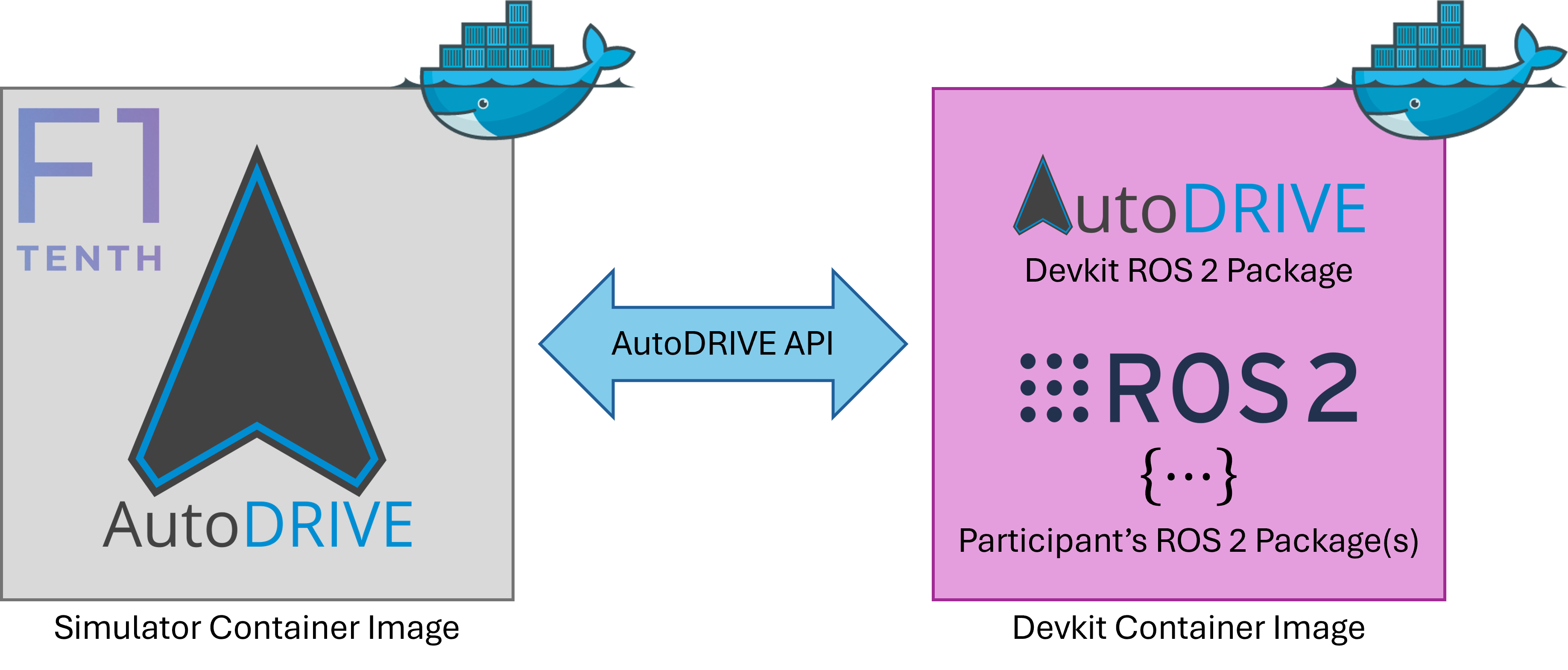
F1TENTH Sim Racing League is a virtual competition, which aims to make autonomous racing accessible to everyone across the globe. This competition adopts a containerization workflow to evaluate the submissions in a reproducible manner. Containerization provides a lightweight and portable environment, allowing applications to be easily packaged along with their dependencies, configurations, and libraries.
Particularly, each team is expected to submit a containerized version of their autonomous racing software stack. Submissions for each phase of the competition will be done separately.
3.1. Container Setup
- Install Docker.
- Since the Docker container is to take advantage of an NVIDIA GPU, the host machine has to be properly configured by installing the necessary NVIDIA GPU Drivers and the NVIDIA Container Toolkit.
- Pull AutoDRIVE Simulator docker image from DockerHub.
- Pull AutoDRIVE Devkit docker image from DockerHub.
Note
Pay close attention to the <TAG> (i.e., tag name) of the container image you are pulling. This could be explore for exploring the framework, practice for practicing and qualification, or compete for competing in the final race. The tag naming convention is set to <YEAR>-<EVENT>-<PHASE> for convenience and avoiding any repetition.
3.2. Container Execution
- Enable display forwarding for simulator:
- Run the simulator container at
entrypoint: - [OPTIONAL] Start additional bash session(s) within the simulator container (each in a new terminal window):
- Enable display forwarding for devkit:
- Run the devkit container at
entrypoint: - [OPTIONAL] Start additional bash session(s) within the devkit container (each in a new terminal window):
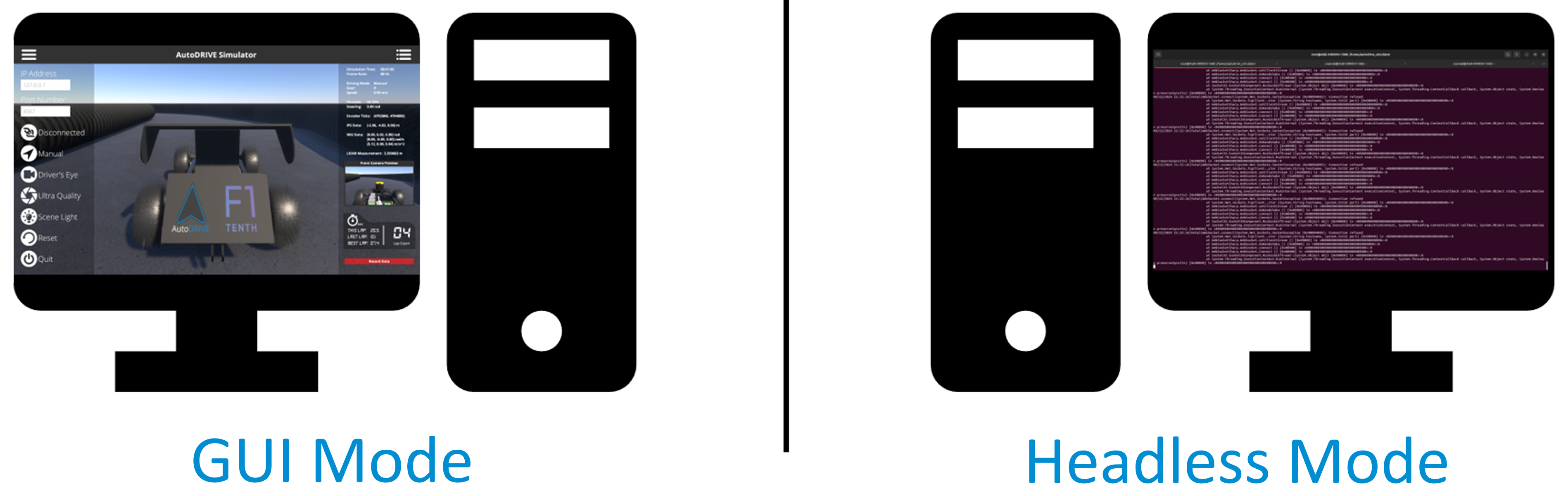
3.2.1. GUI Mode Operations:
- Launch AutoDRIVE Simulator in
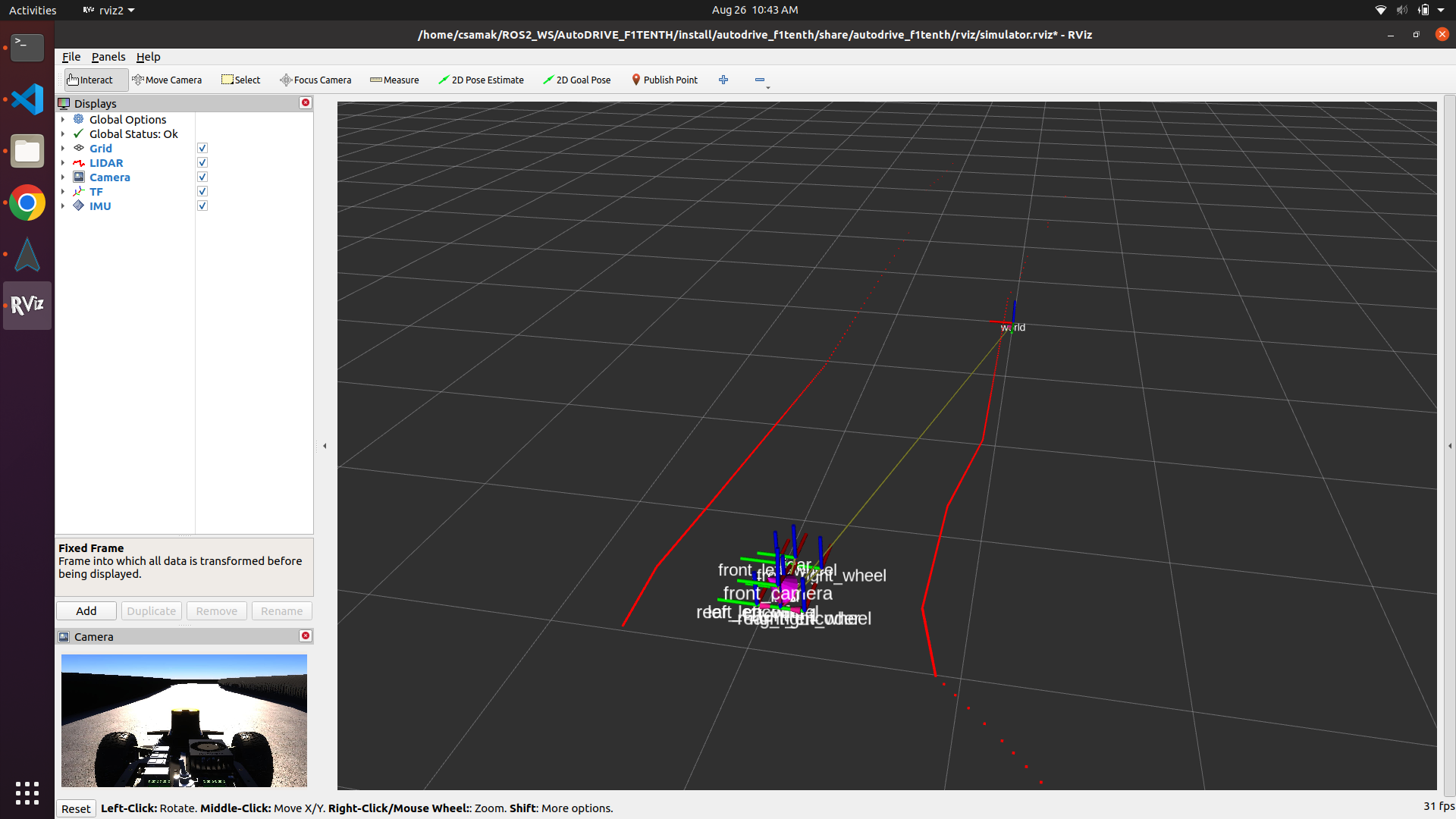
graphicsmode (camera rendering will be enabled): - Launch AutoDRIVE Devkit in
graphicsmode (RViz rendering will be enabled): -
Using the simulator GUI menu panel, configure the following:
3.1. Enter the IP address of the machine running the devkit. If both containers are running on the same machine, leave the default loopback IP.
3.2. Hit the
Connectionbutton and note the status next to it (also note that the devkit echoesConnected!message).3.3. Once the connection has been established, hit the
Driving Modeto toggle the vehicle betweenManualandAutonomousdriving modes.
3.2.2. Headless Mode Operations:
- Launch AutoDRIVE Simulator in
no-graphicsmode (all rendering including vehicle camera will be disabled) by passing the IP address of the machine running the devkit as AutoDRIVE CLI arguments: - Launch AutoDRIVE Simulator in
headlessmode (all rendering except vehicle camera rendering will be disabled) by passing the IP address of the machine running the devkit as AutoDRIVE CLI arguments: - Launch AutoDRIVE Devkit in
headlessmode (RViz rendering will be disabled):
Info
It is possible to run either the simulator, devkit, or both selectively in either graphics or headless/no-graphics mode.
3.2.3. Distributed Computing Mode:

It is possible to run the simulator and devkit on two separate computing nodes (e.g. two different PCs) connected via a common network. The benefit of this approach is workload distribution by isolating the two computing processes, thereby gaining higher performance. It is further possible to run the devkit on a physical F1TENTH vehicle (using the Jetson SBC onboard) and connect it to the PC running AutoDRIVE Simulator as a hardware-in-the-loop (HIL) setup.
Tip
In certain cases, GPUs and Docker do not work very well and can cause problems in running the simulator container. In such cases, you can download and run the simulator locally (it should be easier to access the GPU this way). You can then run only the devkit within a container. Everything else will work just fine, only that the simulator will not be running inside a container. This shouldn not matter, since you will have to submit only the container for your algorithms (i.e., devkit) and not the simulator. We will run the containerized simulator on our side for the evaluation of all submissions.
3.3. Container Troubleshooting
- To access the container while it is running, execute the following command in a new terminal window to start a new bash session inside the container:
- To exit the bash session(s), simply execute:
- To kill the container, execute the following command:
- To remove the container, simply execute:
- Running or caching multiple docker images, containers, volumes, and networks can quickly consume a lot of disk space. Hence, it is always a good idea to frequently check Docker disk utilization:
- To avoid utilizing a lot of disk space, it is a good idea to frequently purge docker resources such as images, containers, volumes, and networks that are unused or dangling (i.e. not tagged or associated with a container). There are several ways with many options to achieve this, please refer to appropriate documentation. The easiest way (but a potentially dangerous one) is to use a single command to clean up all the docker resources (dangling or otherwise):
- After Docker Desktop is installed, Docker CLI commands are by default forwarded to Docker Desktop instead of Docker Engine, and hence you cannot connect to the Docker daemon without running Docker Desktop. In order to avoid this, just switch to the
defaultDocker context:
Warning
It is not recommended to use Docker Desktop on the Linux operating system. This is because Docker Desktop creates a virtual machine based on Linux, which is first of all not needed for native (host) Linux OS, and secondly, it sometimes does not expose the necessary access ports for the containers (e.g., trouble with GPU access).
Info
For additional help on containerization, visit docker.com. Specifically, the documentation and get started pages would be of significant help for the beginners. Also, this cheatsheet could be a very handy reference for all important Docker CLI commands.
3.4. Algorithm Development
Teams will have to create their ROS 2 package(s) or meta-package(s) for autonomous racing within the devkit container separate from the provided autodrive_f1tenth package (i.e., without making any modifications to the autodrive_f1tenth package itself).
Please make a note of the data streams mentioned above (along with their access restrictions) to help with the algorithm development process.
Tip
If working with containers is overwhelming, you can download and run the devkit locally while developing and testing your autonomous racing algorithms. You can then containerize the refined algorithms, test them one last time, and push them to the container registry.
3.5. Container Submission
Note
We expect that upon running your submitted container, all the necessary nodes should start up (the autodrive_devkit API we have included as well as your team's racing stack). Once we hit the Connection Button on the Menu Panel of AutoDRIVE Simulator, the simulated vehicle should start running. Please refer to the competition rules, where it talks about the submission guidelines. Please make sure that you include all the necessary commands (for sourcing workspaces, setting environment variables, launching nodes, etc.) within the entrypoint script (autodrive_devkit.sh file) provided within the autodrive_f1tenth_api container. Please do NOT use ~/.bashrc or other means to automate the algorithm execution! Competition organizers should be able to start additional bash session(s) within your submitted container (without your codebase executing every time a new bash session is initialized) for data recording and inspection purposes.
- Run the image you created in the previous step inside a container:
- In a new terminal window, list all containers and make a note of the desired
CONTAINER ID: - Commit changes to DockerHub:
- Login to DockerHub:
- Push the container to DockerHub, once done, you should be able to see your repository on DockerHub:
- Submit the link to your team's DockerHub repository via a secure Google Form.
4. Citation
We encourage you to read and cite the following papers if you use any part of the competition framework for your research:
AutoDRIVE: A Comprehensive, Flexible and Integrated Digital Twin Ecosystem for Enhancing Autonomous Driving Research and Education
@article{AutoDRIVE-Ecosystem-2023,
author = {Samak, Tanmay and Samak, Chinmay and Kandhasamy, Sivanathan and Krovi, Venkat and Xie, Ming},
title = {AutoDRIVE: A Comprehensive, Flexible and Integrated Digital Twin Ecosystem for Autonomous Driving Research & Education},
journal = {Robotics},
volume = {12},
year = {2023},
number = {3},
article-number = {77},
url = {https://www.mdpi.com/2218-6581/12/3/77},
issn = {2218-6581},
doi = {10.3390/robotics12030077}
}
AutoDRIVE Simulator: A Simulator for Scaled Autonomous Vehicle Research and Education
@inproceedings{AutoDRIVE-Simulator-2021,
author = {Samak, Tanmay Vilas and Samak, Chinmay Vilas and Xie, Ming},
title = {AutoDRIVE Simulator: A Simulator for Scaled Autonomous Vehicle Research and Education},
year = {2021},
isbn = {9781450390453},
publisher = {Association for Computing Machinery},
address = {New York, NY, USA},
url = {https://doi.org/10.1145/3483845.3483846},
doi = {10.1145/3483845.3483846},
booktitle = {2021 2nd International Conference on Control, Robotics and Intelligent System},
pages = {1–5},
numpages = {5},
location = {Qingdao, China},
series = {CCRIS'21}
}